Phonon Dispersion

This example is originally from GPUMD and has been added here with minor changes only to demonstrate how to use gpyumd.

1. Introduction

• In this example, we use harmonic lattice dynamics to calculate the phonon dispersion of diamond silicon.

Importing Relevant Functions

• The inputs/outputs for GPUMD are processed using the Atomic Simulation Environment (ASE) and the gpyumd package.

import matplotlib.pyplot as plt
from ase.lattice.cubic import Diamond
from ase.build import bulk
from gpyumd.atoms import GpumdAtoms
from gpyumd.sim import Simulation
import gpyumd.keyword as kwd
from gpyumd.load import load_omega2

2. Preparting the Inputs

• The structure as specified is 64-atom diamond silicon at zero temperature and zero pressure.

• Weuse the minimal Tersoff potential [Fan 2020].

Create Si Unit Cell & Add Basis

a=5.434
Si_UC = GpumdAtoms(bulk('Si', 'diamond', a=a))
Si_UC.add_basis()
Si_UC

GpumdAtoms(symbols='Si2', pbc=True, cell=[[0.0, 2.717, 2.717], [2.717, 0.0, 2.717], [2.717, 2.717, 0.0]])

The xyz.in file

Transform Si to cubic supercell first. Note: We write the xyz.in file here for demonstration purposes, but the Simulation we are about to make also outputs the xyz.in file.

# Create 8 atom diamond structure
Si = Si_UC.repeat([2,2,1])
Si.set_cell([a, a, a])
Si.wrap()

# Complete full supercell
Si = Si.repeat([2,2,2])
Si.set_max_neighbors(4)
Si.set_cutoff(3)
Si.write_gpumd()
Si

GpumdAtoms(symbols='Si64', pbc=True, cell=[10.868, 10.868, 10.868])

The basis.in file

Si.write_basis()

• The basis.in file reads:

  2
  0 28.085
  1 28.085
  0
  1
  0
  1
  0
  1
  ...
  

• Here the primitive cell is chosen as the unit cell. There are only two basis atoms in the unit cell, as indicated by the number 2 in the first line.

• The next two lines list the indices (0 and 1) and masses (both are 28.085 amu) for the two basis atoms.

• The next lines map all the atoms (including the basis atoms) in the super cell to the basis atoms: atoms equivalent to atom 0 have a label 0, and atoms equivalent to atom 1 have a label 1.

The kpoints.in file

• The \(k\) vectors are defined in the reciprocal space with respect to the unit cell chosen in the basis.in file.

• We use the \(\Gamma-X-K-\Gamma-L\) path, with 400 \(k\) points in total.

linear_path, sym_points, labels = Si_UC.write_kpoints(path='GXKGL',npoints=400)

The run.in file

The gpyumd package can be used to generate valid run.in input files as well as other necessary input files. It follows the definitions described in the inputs and outputs documentation for GPUMD.

phonon_sim = Simulation(Si, driver_directory='.')
phonon_sim.add_static_calc(kwd.ComputePhonon(cutoff=5, displacement=0.005))
potential_directory = "C:/Users/gbear/Documents/CUDA_Dev/GPUMD/potentials/tersoff"
tersoff_potential = \
    kwd.Potential(filename='Si_Fan_2019.txt', symbols=['Si'], directory=potential_directory)
phonon_sim.add_potential(tersoff_potential)
phonon_sim.create_simulation(copy_potentials=True)

The run.in input file is given below:

potential Si_Fan_2019.txt 0

compute_phonon 5 0.005

• The first line with the potential keyword states that the potential to be used is specified in the file Si_Fan_2019.txt.

• The second line with the compute_phonon keyword tells that the force constants will be calculated with a cutoff of 5.0 \(\mathring A\) (here the point is that first and second nearest neighbors need to be included) and a displacement of 0.005 \(\mathring A\) will be used in the finite-displacement method.

3. Results and Discussion

Figure Properties

aw = 2
fs = 16
font = {'size'   : fs}
plt.rc('font', **font)
plt.rc('axes' , linewidth=aw)

def set_fig_properties(ax_list):
    ax_list = ax_list if isinstance(ax_list, list) else [ax_list]
    tl = 8
    tw = 2
    tlm = 4

    for ax in ax_list:
        ax.tick_params(which='major', length=tl, width=tw)
        ax.tick_params(which='minor', length=tlm, width=tw)
        ax.tick_params(which='both', axis='both', direction='in', right=True, top=True)

Plot Phonon Dispersion

• The omega2.out output file is loaded and processed to create the following figure. The previously defined kpoints are used for the \(x\)-axis.

nu = load_omega2()

plt.figure(figsize=(10,10))
set_fig_properties(plt.gca())
plt.vlines(sym_points, ymin=0, ymax=17)
plt.plot(linear_path, nu, color='C0',lw=3)
plt.xlim([0, max(linear_path)])
plt.gca().set_xticks(sym_points)
plt.gca().set_xticklabels([r'$\Gamma$','X', 'K', r'$\Gamma$', 'L'])
plt.ylim([0, 17])
plt.ylabel(r'$\nu$ (THz)')
plt.show()

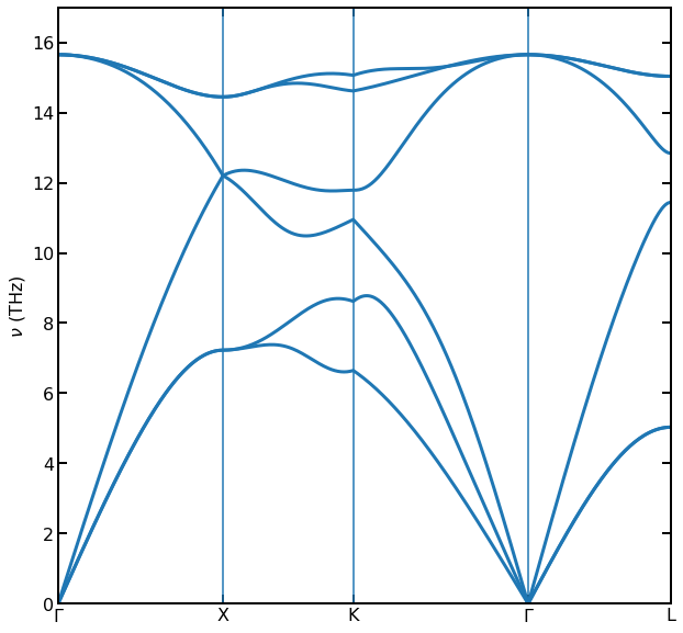
Phonon dispersion of silicon crystal described by the mini-Tersoff potential.

• The above figure shows the phonon dispersion of silicon crystal described by the mini-Tersoff potential [Fan 2020]

4. References

[Fan 2020] Zheyong Fan, Yanzhou Wang, Xiaokun Gu, Ping Qian, Yanjing Su, and Tapio Ala-Nissila, A minimal Tersoff potential for diamond silicon with improved descriptions of elastic and phonon transport properties, J. Phys.: Condens. Matter 32 135901 (2020).